

What Die Casting Flow Simulation Actually Predicts: Fill, Air Entrapment, and Thermal Balance
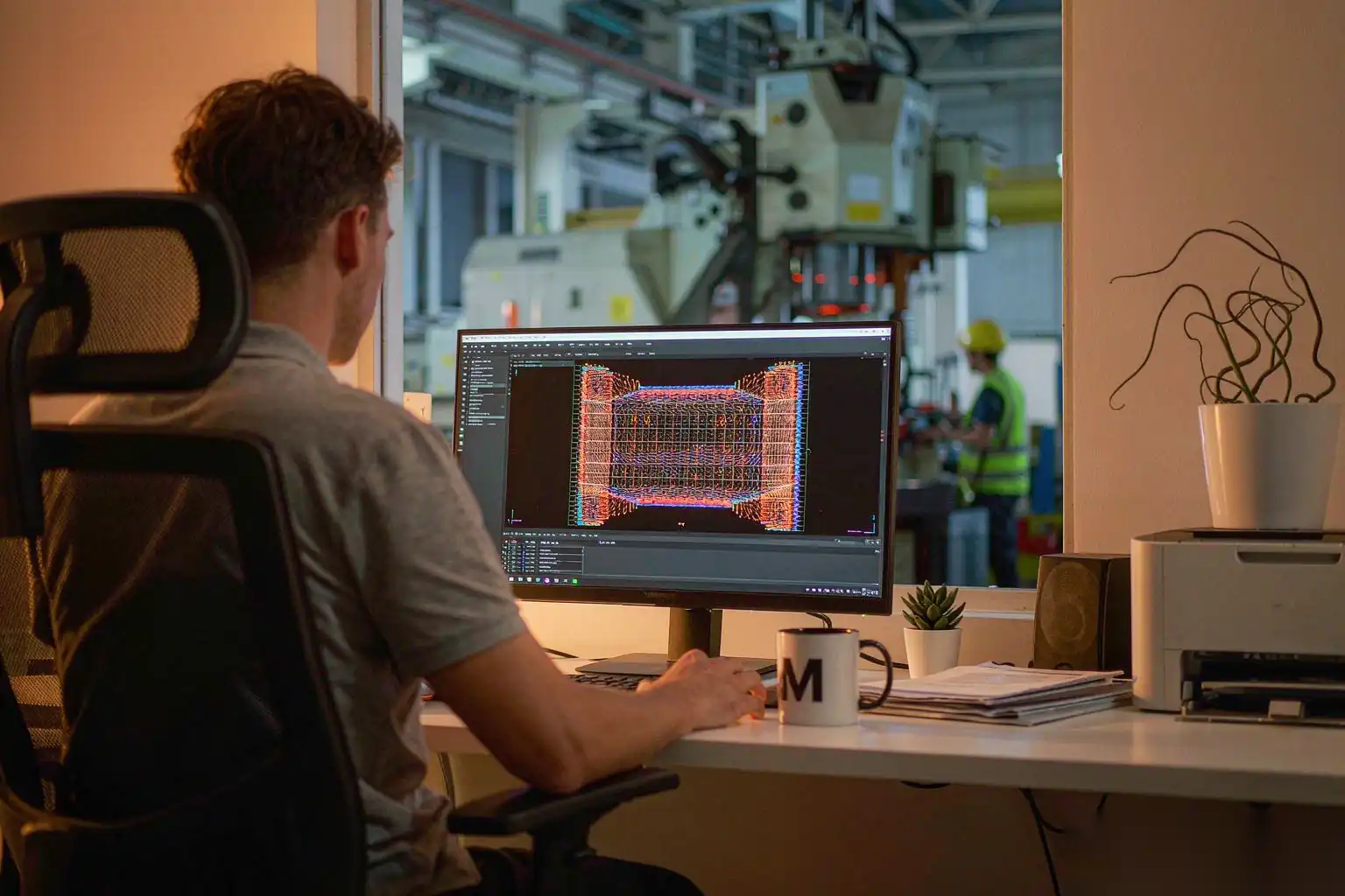
We run fill simulation on most die casting programs before any steel is cut, and we still watch teams treat the colour animation as a certificate of approval. It is not a certificate. A fill model is a numerical experiment that answers a narrow set of questions about metal front behaviour inside a closed cavity — behaviour that no production sensor can observe directly. Handled that way, it regularly removes two or three tool trials from a program. Handled as decoration, it produces a convincing animation that has little to do with the casting in your hand.
This piece sets out what we ask a fill model to predict, which inputs decide whether the answer is worth paying for, how to turn the output into geometry and process changes, and where the method stops.
Where a Fill Model Earns Its Keep
The economic case is simple. A mid-size aluminium tool for a 1.5 kg housing costs a serious sum and carries a lead time measured in weeks, and every geometry change after first steel costs both. Simulation is cheap relative to steel. The programs where it pays hardest share clear characteristics:
- Large or thin-wall parts where fill time is long relative to solidification time. Thin walls below 1.5 mm over a flow length beyond 250 mm are the classic case.
- Parts with cosmetic or pressure-tight surfaces, where the location of last fill and oxide accumulation decides whether the part can be finished at all.
- Multi-cavity or family tools where balance between cavities cannot be trimmed by eye.
- Parts machined on sealing faces, where porosity at a specific depth below a boss matters more than average porosity.
The programs where it pays least are equally clear: a small single-cavity part with generous wall thickness, well-established gating, and no cosmetic or leak requirement. There, an experienced toolmaker beats a model built on guessed inputs.
Inputs That Decide Whether the Model Is Worth Anything
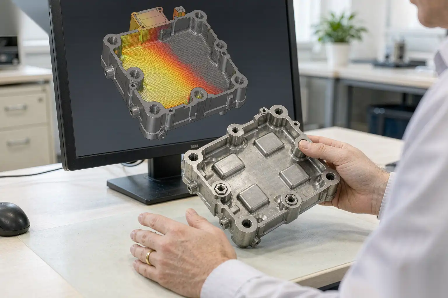
Solver accuracy is rarely the limiting factor. Input quality is. A model run with catalogue alloy data, an isothermal die, and a constant-velocity plunger will produce smooth, plausible, and wrong results. Four input groups dominate the outcome.
Alloy data and thermal properties
Use measured or alloy-supplier-specific data, not a generic default. For ADC12 and A380-type alloys, the numbers that matter are liquidus and solidus (roughly 580 °C and 515 °C for the Al-Si-Cu family), latent heat, specific heat, thermal conductivity in both liquid and solid state, and — the one almost always skipped — viscosity as a function of solid fraction. Above about 20 percent solid fraction the effective viscosity rises steeply, and that rise is what stops a front in a thin rib. Density change on solidification drives the feeding calculation in solidification runs.
Pouring temperature should be the temperature in the shot sleeve, not the furnace setpoint. A holding furnace at 680 °C feeding through a transfer ladle routinely delivers 650 to 660 °C at the sleeve. That 20 to 30 °C moves predicted cold shut risk measurably on thin sections.
Die thermal profile
A die run is not isothermal. The steady-state die surface temperature depends on local heat flux, cooling channel layout, and cycle time. We normally ask for three conditions: shot 1, shot 15, and steady state at the production cycle time. A cold-start run with the die at ambient gives a pessimistic fill picture that no production part sees after the first ten shots. Cooling line flow rates, inlet temperature, and whether a channel is actually flowing — many are choked or scaled — must be entered as built, not as designed.
Spray and lubricant film
Water-based die lubricant leaves a film whose local thickness and residual water govern interfacial heat transfer. In practice the heat transfer coefficient between casting and die varies by roughly a factor of three between a heavy spray zone and a wiped-dry zone. Where an operator dwells with the spray gun changes fill balance between cavities. If a program has a known hot spot, simulate both a nominal film and a locally heavy film; the sensitivity tells you how much process drift the design tolerates before it produces scrap.
Plunger law
Fill simulation is only as good as the plunger velocity profile fed into it. Three things are needed: slow-shot velocity, fast-shot velocity, and switch point position. The slow shot must stay below the critical velocity at which a wave forms and air is folded in the sleeve — typically in the 0.2 to 0.5 m/s band for a 60 to 80 mm sleeve, calculated from sleeve diameter and fill level. Fast-shot velocity follows from gate area and target fill time:
- Fill time target for a 2 to 3 mm wall cosmetic aluminium part: 40 to 80 ms.
- Gate velocity at the ingate: normally 30 to 60 m/s, and deliberately lower, 20 to 35 m/s, where the gate discharges directly against a cavity wall or a core.
- Intensification rise time: under 30 ms to set pressure, otherwise the intensifier is pressurising metal that has already frozen at the gate.
Give the analyst the machine’s actual intensification curve, including pressure overshoot. A model that assumes instantaneous pressure build-up will under-predict flash at the parting line, and flash is what drives deburring cost later.
Reading the Results: Six Outputs That Drive Design Changes
Most solvers produce a dozen fields. Six are actionable on a daily basis.
| Output | What it tells you | Threshold we act on |
|---|---|---|
| Front arrival time | Whether each cavity region fills inside the available window | Any region exceeding 100 ms on a 2.5 mm wall |
| Front temperature | Cold shut and misrun risk where fronts meet | Front temperature below liquidus minus 15 °C |
| Air entrapment pressure | Where trapped air is compressed and where it ends up | Predicted pressure above 20 to 30 MPa at a machined face |
| Last-fill location | Where oxide, lubricant residue and gas concentrate | Last fill landing on a cosmetic or sealing face |
| Oxide tracking | Probability of bifilm defects at a given location | Oxide concentration at a tapped hole or seal groove |
| Solidification time | Shrinkage void location and feeding path | Hot spot isolated from the gate by already-frozen metal |
Front arrival time is the one output we insist on seeing as a numbered sequence rather than a colour ramp, because the sequence tells you the merge order. Two fronts meeting at 40 ms with both above 600 °C will weld acceptably. The same two fronts meeting at 80 ms, with one at 570 °C, produce a visible cold shut line that no amount of polishing removes cleanly, because the line is an oxide film folded into the surface. Grinding it out leaves a shadow that reappears under anodising or plating.
Air entrapment results have to be read together with the venting design. A trapped pocket next to a functioning overflow and vent is a minor issue. The same pocket in a dead corner with no escape path becomes a gas pore at 0.5 to 1.5 mm below the surface, which is exactly the depth a CNC facing cut will open.
Acting on the Results: Gate, Overflow, Vent, Plunger
Simulation output is worthless unless it changes geometry or process. Four levers, in our order of preference:
- Gate relocation. Moving the ingate changes the whole flow map and is best done before steel is cut. If last fill sits on a cosmetic face, the fix is usually to feed from the opposite end, or to add a second gate so that fronts meet over an overflow rather than over the visible surface.
- Overflow placement. Overflows are not just scrap collectors. Positioned at predicted last-fill and oxide accumulation zones, they pull cold, dirty metal out of the casting. Volume matters: an overflow sized at 20 to 30 percent of the local casting volume does real work, while a token 5 percent slug adds trim cost and does nothing.
- Venting. Vent cross-section should be sized from the evacuation requirement, not copied from the previous tool. As a working rule, vent area in the range of 0.1 to 0.3 percent of projected cavity area per vent run, with a land length of 0.5 to 1.0 mm before the relief channel. Chill vents and vacuum assistance extend the same logic.
- Plunger profile change. A new fast-shot velocity or switch point costs an hour of press time and no steel. If the model shows wave formation in the sleeve, the fix is a lower slow-shot velocity, a larger sleeve fill ratio, or a switch point further along. If it shows a front stalling in a thin rib, the fix may be a higher fast-shot velocity, a hotter die, or a locally thickened section — never all three at once, or you will never know which one worked.
One caution on iterating. Change one variable per run and keep a log. We have seen programs where six simultaneous improvements produced a worse part than the baseline and nobody could say which change hurt.
Mesh and Modelling Setup: Practical Numbers
Cell size defines both cost and resolution. For a typical 300 × 250 × 80 mm housing we use a body cell of 1.5 to 2.0 mm, refined to 0.8 to 1.0 mm through wall thickness transitions and to 0.5 mm at gates and vents. That gives 3 to 5 cells through a 2.5 mm wall, enough to resolve the solidification gradient and not enough to resolve surface tension effects, which the model does not attempt anyway.
Practical setup notes:
- Model the shot sleeve, biscuit and runner, not just the cavity. Air folded in the sleeve arrives in the cavity and shows up as porosity.
- Include overflows and vents in the mesh. Excluding them removes the escape path and over-predicts air pressure.
- Include cores and slides as heat sinks with their own material properties. Tool steel inserts with internal cooling behave very differently from solid steel blocks.
- Run at least 5 to 8 cycles in the thermal model to reach a repeatable die temperature before judging the fill result. Single-shot thermal results are misleading.
- Let the solver set the time step from the Courant condition. Overriding it to speed up a run costs accuracy you cannot see in the plot.
What Simulation Cannot Predict
This is the section that gets skipped, and it is where most disappointment originates.
- Die soldering and washout. Local metal attack on a core is driven by lubricant chemistry and die surface condition, neither of which a flow model represents.
- Lubricant-related cosmetics. Flow marks, drag marks and spray swirl are not captured by a single interfacial heat transfer coefficient.
- Ejection distortion. Fill and solidification models stop at die open. Ejection stress and the warp that follows need a separate structural analysis with temperature-dependent material data.
- Blistering during heat treatment or painting. The model tells you where gas is and at what pressure. It does not tell you whether that gas will expand into a blister at 480 °C solution treatment or at 200 °C powder cure. That correlation has to be built from your own parts.
- Statistical variation. A deterministic run gives one answer. Production varies plunger velocity by roughly ±3 percent, die temperature by ±15 °C, and alloy composition within specification. If a design sits close to a threshold, run a sensitivity band instead of trusting one plot.
Validation Against Real Castings
We treat the first simulation as a hypothesis. The validation loop we run at T1:
- Short-shot series. Stop the plunger at 30, 50, 70, 85 and 100 percent of stroke and compare the short shots against the predicted front arrival sequence. If the sequence matches, the flow map is trustworthy. If the model says the front reaches a boss before a nearby rib and the short shot shows the opposite, the inputs are wrong, usually gate area or plunger velocity.
- Dye penetrant or vacuum impregnation on machined faces. Compare predicted gas pressure locations against actual leak points.
- Sectioning and porosity measurement. Cut the predicted worst location, polish, and measure pore size and area fraction. If the model says 3 percent porosity and you measure 0.3 percent, the air entrapment boundary conditions are pessimistic. Recalibrate rather than discarding the model.
- Thermal imaging of the die face. A steady-state infrared image at production cadence validates the die thermal profile, which is the input most likely to have drifted from design intent.
Record the comparison in a one-page table in the program file. Six months later, when someone asks why a gate was moved, the answer should not be a recollection.
How Simulation Evidence Shortens the T1-to-Approval Loop
The mechanism is not that simulation makes the first part perfect. It is that simulation converts an argument into a decision. Without a model, a T1 review is a negotiation between the toolmaker, the foundry and the customer’s engineer about whose experience applies. With a model plus short-shot validation, the same meeting has a shared picture of where the metal went and why the pore is where it is.
In practice we see three effects. Gate and overflow decisions move earlier, into the design phase, so first steel is closer to final. Process windows get documented before production starts, meaning a defined fast-shot velocity, switch point and die temperature band rather than whatever the operator found in week one. And downstream finishing is planned with knowledge of where surface defects will land. If the model says last fill and oxide accumulation sit on the flange face that will be robotically ground and polished, the finishing cell can be specified for that removal depth from the start, instead of being retrofitted after the first batch comes back with visible lines.
That last point touches our own work directly. Surface condition at the casting stage sets the cost of everything downstream: a cold shut line that survives into the finishing cell has to be ground out, and grinding out a line means removing metal, holding tolerance and accepting a longer cycle. If you want to see how casting surface condition converts into finishing cost, read our breakdown of aluminum die casting finishing options and the companion discussion in aluminum die casting defects and solutions. Porosity location matters just as much, and aluminum die casting porosity causes and solutions covers what happens when those predicted gas pockets are opened by a machining cut.
Die casting flow simulation is a tool for reducing unknowns before committing to steel. Its value is proportional to the honesty of its inputs and the discipline of its validation. Run it as an experiment, check it against short shots, and it pays for itself in tool trials you never had to run.
DZ Machinery builds robotic deburring, grinding and polishing cells for die cast and faucet hardware, and we regularly review casting simulation output with customers before specifying a finishing process. If you are planning a new die cast program, send us the part drawings and the fill model, and we will tell you what the finishing cell will need to remove and what cycle time that implies.