

QUICK FACTS
| Cell footprint | 2.5–6 m² |
| Changeover | <15 min between SKUs |
| Media life | 60–180 parts/belt |
A robotic grinding machine cost conversation usually starts with the quote and ends with a shrug. The quote is real, but the return stays abstract, so the project stalls in a budget meeting. This article fixes the math.
We break the investment into its real components, model the labor and quality offsets with honest numbers, and run three payback scenarios at different production volumes. By the end, the decision becomes arithmetic instead of debate.
What the Investment Actually Contains
The robot arm is rarely the biggest line item. A complete grinding cell bundles several cost blocks, and buyers who model only the robot systematically underestimate by a third. Here is the honest structure.

| Cost Block | Share of Total | Notes |
|---|---|---|
| Robot and controller | 25 – 35% | Reach and payload set the class |
| Process end-effectors | 15 – 25% | Spindles, contact wheels, force control |
| Fixtures and tooling | 10 – 20% | Per part family |
| Guarding and extraction | 10 – 15% | Safety compliance is not optional |
| Integration and programming | 15 – 20% | Often underestimated most |
| Training and commissioning | 5 – 10% | Shortens ramp, pays for itself |
Integration deserves special attention. Connecting the cell to your power, air, and information systems takes engineering hours that appear on the invoice whether you planned them or not. Ask for this line item explicitly in every quote.
The Labor Offset Model
Labor is the obvious saving, but the details decide whether the model survives scrutiny. Count fully loaded wages, not base pay. Add benefits, insurance, and supervision. In most industrial regions a grinding operator costs the company 1.4 to 1.8 times their wage.
Shift coverage multiplies the effect. One operator per shift across two shifts means two positions offset. Across three shifts, three positions. A cell that runs lights-out on the night shift earns savings no daytime hire could match.
Do not forget turnover. Grinding benches lose operators to harder jobs and competitors at rates above plant average. Every replacement carries recruiting and retraining costs. Automation removes that recurring tax from your cost structure.
Quality Gains That Show Up in Money
Grinding quality is not a soft benefit. It lands in three hard accounts. Scrap falls first, because robotic paths remove the same material every cycle instead of depending on how the operator feels that hour.
Rework falls second. Parts that leave the cell within tolerance do not return from inspection. Plants converting from manual grinding typically report rework rates dropping by half or more within the first quarter.
Downstream complaints fall third. A casting with a consistent finish assembles better, coats better, and fails warranty claims less often. Finance teams accept this line once you show historical claim costs, and the numbers are rarely trivial.
Three Worked Payback Scenarios
Models earn trust when the assumptions are visible. Here are three scenarios at different volumes, each using conservative inputs. Adjust the inputs to your rates and the method still holds.
| Scenario | Small Job Shop | Mid-Size Foundry | High-Volume Plant |
|---|---|---|---|
| Cell investment | $180,000 | $260,000 | $420,000 |
| Operator positions offset | 1.0 | 2.0 | 3.0 |
| Loaded labor saving / year | $62,000 | $124,000 | $186,000 |
| Scrap and rework saving / year | $18,000 | $45,000 | $90,000 |
| Consumables and power / year | -$12,000 | -$20,000 | -$34,000 |
| Net annual benefit | $68,000 | $149,000 | $242,000 |
| Simple payback | 2.6 years | 1.7 years | 1.7 years |
The mid-size and high-volume cases converge near 1.7 years because volume amortizes integration cost faster. Small shops should not be discouraged by 2.6 years. Their cells also open capacity that lets the shop quote larger contracts.
Every scenario excludes two upside items on purpose. Overtime reduction and the ability to accept rush orders both add return that only appears after the cell runs. Keep them out of the approval model and enjoy them later.
Sensitivity: What Moves the Payback
Four variables swing the model more than any others. Test each one before you present, because the ownership meeting will test them for you.
Utilization Rate
A cell running sixty percent of available hours earns roughly sixty percent of the modeled saving. Plan loading honestly. If your part flow cannot fill the cell, add families or shift the investment decision a quarter.
Cycle Time Accuracy
Vendor demo cycles are best-case. Real cycles include loading, sensing, and tool compensation. Model your payback at demo time plus fifteen percent and the model survives production.
Fixture Count
Each added part family costs fixtures and programming hours. Families below a volume threshold may never repay their tooling. Rank your families by annual volume and let the ranking, not enthusiasm, set the fixture budget.
Labor Rate Trajectory
Wages in most industrial regions rise three to six percent yearly. A payback modeled at today’s rates improves every year you wait. This is the quiet argument for deciding now rather than next budget cycle.
These sensitivities connect directly to process discipline. A cell that runs optimized parameters hits its modeled cycle times consistently. Our deburring process optimization tips explain the parameter work that keeps real production aligned with the model.
Risks to the Model and How to Retire Them
Every ROI model carries risks, and honest ones name them. Three risks dominate grinding projects. Each has a known retirement strategy that costs less than the risk itself.
Part Variation Exceeds Assumptions
Castings vary, and rigid paths fight variation. The fix is force control or compliance in the end-effector, priced early rather than retrofitted. Cells specified with compensation from day one meet their models; cells specified rigid often do not.
Ramp Takes Longer Than Planned
New cells meet new problems. Budget six weeks of ramp rather than two, and staff the project with your best process person. The labor saving starts slightly later but then holds, and the model barely notices a month.
Skills Gap on the Floor
Cells need operators who can restart programs and swap tools, not just load parts. Training is cheap insurance. Our operator training guide for automated grinding and polishing lays out a four-week program that turns machine attendants into cell owners.
Data Collection During the First Quarter
The first ninety days of cell operation generate the data that either validates or corrects your model. Log cycle times, wheel consumption, reject rates, and downtime reasons from the first shift. Simple spreadsheets beat elaborate systems at this stage, because the habit matters more than the software.
Compare the logged reality against the model monthly, not daily. Daily comparisons chase noise; monthly ones reveal drift. Where reality beats the model, update the forecast and enjoy the credibility. Where it lags, find the line item and fix the cause while the project still has momentum.
Presenting the Model to Ownership
Ownership meetings reward clarity. Lead with the payback number and the utilization assumption behind it. Show the sensitivity table second. Keep the technical appendix for the engineers who ask, because most approvers want the shape of the decision before the depth.
One page works. Investment, savings structure, payback range, and the three risks with their fixes. If the one page survives questions, the project has a real chance. If it cannot be written on one page, the model is not ready.
Teams comparing automation against manual methods across the whole plant should also read our robotic versus manual grinding cost comparison for 2026, which extends this model to the full shop-floor economics.
Energy and Consumables in the Operating Budget
Operating costs deserve their own line of sight. A grinding cell draws meaningful power during contact, but idle draw matters too. Modern cells that park the spindle between parts cut idle consumption sharply, and that difference shows up monthly.
Abrasives are the bigger recurring item. Wheel spend scales with removed volume, not with machine hours, so parts with heavy stock allowances consume more. Log wheel changes per hundred parts from week one and the consumption model becomes real data within a quarter.
Coolant and dust disposal add modest but permanent costs. Neither is large enough to break the model, yet both belong in it. A model that survives an audit is built from line items, and finance reviewers notice the difference.
The Second Cell Discount
Plants rarely stop at one cell. The first cell teaches lessons that make the second cheaper in three concrete ways. Fixtures arrive faster because the fixture design language already exists. Programming time drops because path templates transfer between families.
Most importantly, your team stops needing vendor hand-holding for routine items. The second project usually runs twenty to thirty percent cheaper on integration and commissioning combined. Approving cell one is therefore also approving a discount on cell two.
The Decision Arithmetic
Robotic grinding machine cost stops being intimidating when the return side gets the same rigor as the quote side. Build the model from the cost blocks, run your volumes through the three scenarios, and stress-test the four sensitivities.
Plants that follow this sequence report a consistent outcome. The cell earns its payback near the modeled date, the quality savings arrive as predicted, and the second cell gets approved faster than the first. That is what disciplined ROI math actually buys.
Run the numbers with your real rates this week. The arithmetic has a way of making the decision obvious.
Figures are illustrative; actual results depend on part geometry, material, and cell configuration.